Food Manufacturing Financial Model in Quantrix: From 4 to 20 Products Without Changing a Formula
This food manufacturing financial model plans 20 products in four product families, made in four plants and sold in eight regions, over five years and three scenarios. It started with four products, two plants and three regions. We scaled it up five-fold without changing a single formula: the model has 74 formulas before and after. It is built in Quantrix and you can get it free with the 30-day Quantrix trial. All names and figures in the model are fictitious.
Can a financial model grow from 4 to 20 products without new formulas?
Most Excel models that become unmanageable did not start that way. They started with a few products and one plant, then every new product, plant, region or year meant another copied sheet, another set of links and another place for a mistake. We did the opposite test with this model: we added items and data, and nothing else.
| Before | After | |
|---|---|---|
| Products | 4 | 20, in 4 families |
| Plants | 2 | 4 |
| Sales regions | 3 | 8 |
| Raw materials | 5 | 10 |
| Years | 3 | 5 |
| Scenarios | 3 | 3 |
| Formulas | 74 | 74 |
| Calculated values | 1,836 | 18,618 |
| Matrices | 25 | 25 |
| Model checks | pass | pass |
The model has ten times as many calculated values and exactly the same formulas. Every check in the model’s control layer passes in all three scenarios and all five years: production volume equals volume sold, the P&L reconciles to its components, plant allocation weights add up to 100%, and revenue by product family adds up to company revenue.
Why did no formula have to change?
Because a Quantrix formula refers to names, not cells, and is written once for a whole dimension. This is the revenue formula in the model:
Revenue EUR = round(Calc_Regional_Volume::Regional Volume Tonnes * Selling Price Per Tonne, 0)It calculates revenue for every product, region, year and scenario. With 4 products it produced 108 values; with 20 products it produces 2,400. When a product, a region or a year is added, the formula already covers it. The same is true for the bill of materials, conversion cost, the COGS waterfall, the P&L and the checks.
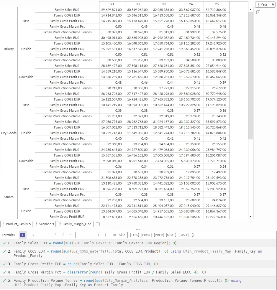
Product families work the same way. Which family a product belongs to is not written into any formula. It is a mapping table of 20 rows, Bread to Bakery, Ketchup to Sauces and so on, and one formula sums revenue, cost and volume by family through that table. Moving a product to another family is a data change.
The idea behind this, one model with linked dimensions instead of one sheet per unit, is explained in multidimensional financial modelling. This page shows what it means in numbers.
What would the same model look like in Excel?
In Excel, every calculated value is its own formula cell, even when it is a copy. The same model would need 18,618 formula cells, about 250 for each Quantrix formula. The number of sheets depends on the layout. We assumed a common one: years across the columns, one sheet per product and scenario for the product calculations, and one sheet per scenario for each company-level block such as the P&L, overheads, product families and checks.
| Quantrix | Excel, layout as described | |
|---|---|---|
| Formulas to write and maintain | 74 | 18,618 formula cells |
| Sheets or matrices | 25 matrices | about 87 sheets (60 product sheets, 27 company-level) |
| Add one product | add the item and its data; 0 formula changes | 840 new formula cells, 3 new sheets, links into every total |
| Compare scenarios side by side | a view of the same model | three copies of the calculation sheets |
An Excel modeller could cut the sheet count to about 30 with a scenario switch, at the price of seeing only one scenario at a time. A real budget is usually much larger than this demonstration: OYAK Beton’s Excel budget had grown to more than 150 spreadsheets in 10 files before it became one Quantrix model.
What is in the model?
- Products and families: 20 products in Bakery, Dry Goods, Sauces and Snacks, from bread and pasta to ketchup and wafers
- Plants: four plants; each product is made in a main plant and a second plant
- Regions: eight sales regions, supplied from the plants through allocation weights
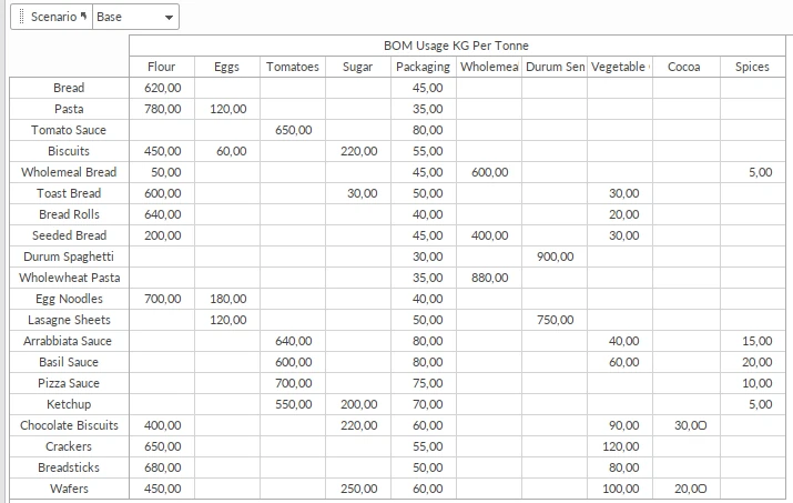
- Raw materials: ten, from flour and durum semolina to cocoa and packaging, with a bill of materials per product
- Time and scenarios: five years; Base, Upside and Downside
- Currency: euros
Which assumptions can you change?
- Volumes: production volume by product and plant in the base year, and how each plant’s output is split across the regions
- Prices: selling price per tonne by product and region
- Costs: bill of materials, raw material prices per kg, conversion cost per tonne by product and plant (labour, energy, line costs), fixed overhead, SGA and depreciation
- Scenario drivers by year: volume growth, raw material inflation, price increase, overhead growth, CPI, corporate tax rate and depreciation growth
- Product families: the mapping of each product to its family
What does it calculate?
- production volume by product, plant and year, and volume sold by region
- revenue by product and region
- raw material cost from the bill of materials, with raw material inflation, and conversion cost by plant
- a COGS waterfall for every product: raw materials at base-year prices, the inflation effect, conversion cost
- revenue, gross and contribution margin per tonne by product
- revenue, COGS, gross margin and volume by product family
- a consolidated P&L from revenue to EBITDA, EBIT and NOPAT, and a KPI dashboard
- a control layer of six checks with a PASS or REVIEW status in every scenario
What does the model show?
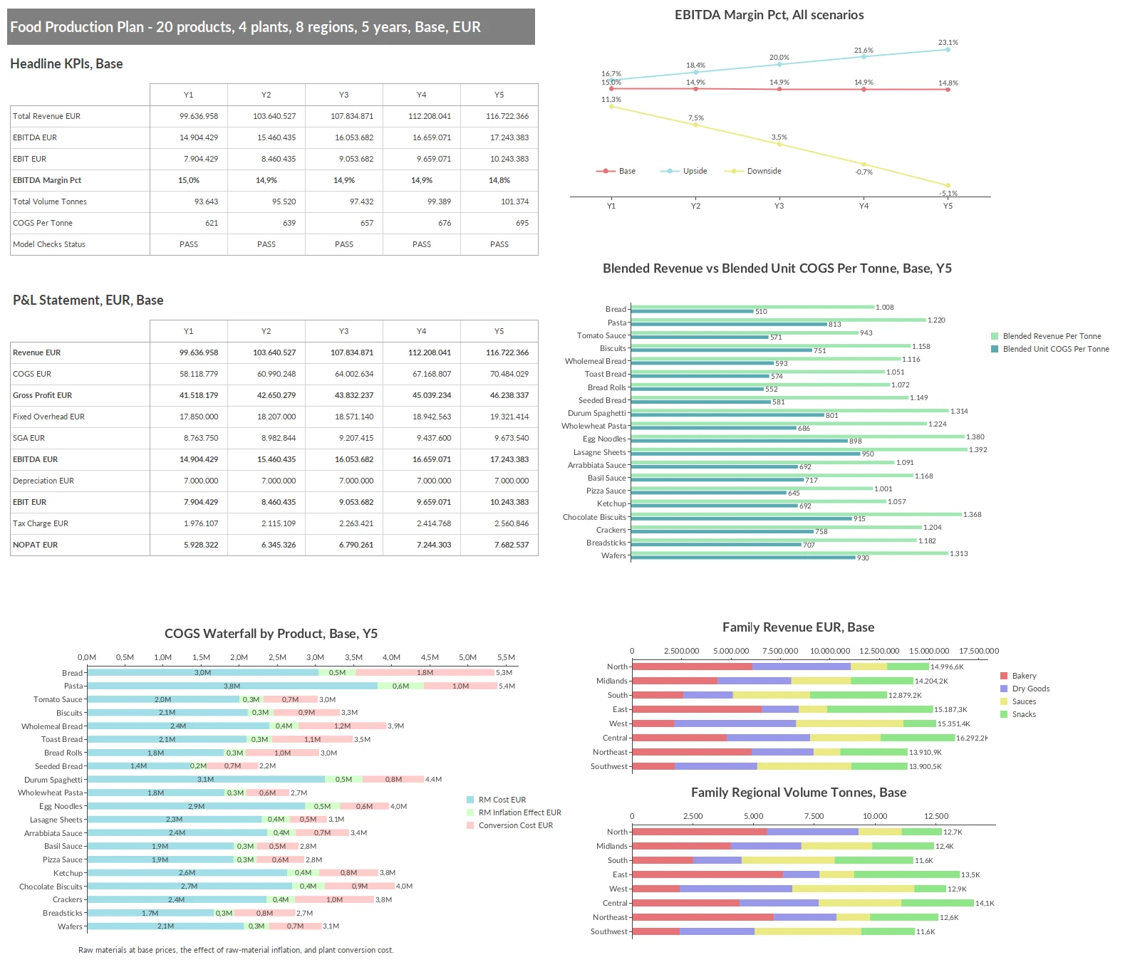
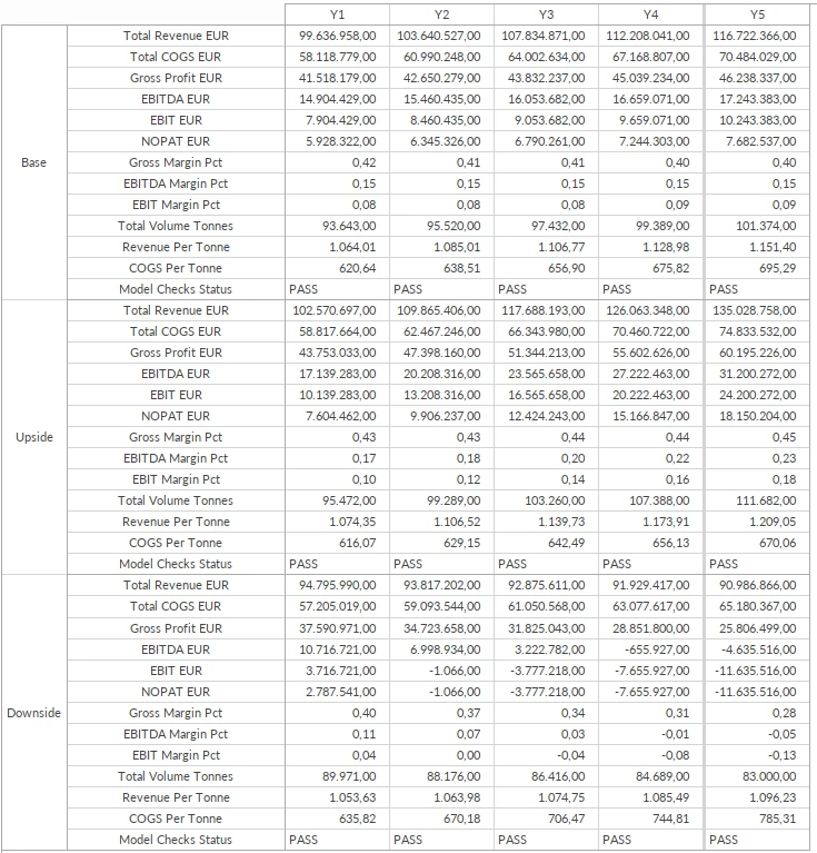
In the Base scenario revenue grows from €99.6 million in year 1 to €116.7 million in year 5, and EBITDA margin holds at about 15%. In the Upside scenario stronger volume and prices lift EBITDA margin to 23.1% by year 5.
The Downside scenario shows operating leverage. Raw material prices rise 6% a year while selling prices rise only 1%, and volume falls 2% a year against fixed overheads that keep growing. EBIT is already slightly negative in year 2, EBITDA turns negative in year 4, and by year 5 the operating loss (EBIT) reaches €11.6 million. The model shows where it comes from, product by product and plant by plant.
By product family, Bakery earns the highest gross margin, about 50% in the Base scenario. In the Downside scenario Bakery still holds 39% in year 5, while Dry Goods, Sauces and Snacks each lose about 12 percentage points and end between 23% and 25%.
How was this model built?
It was generated from a plain-language brief with our AI Quantrix model builder, then reviewed and tested; every figure on this page was checked against an independent recalculation. The scale-up was done in two steps: first the logic, so that no formula names a specific product, plant or region; then the new items and their data.
What the model does not include
The demonstration model stays at operating P&L level so the logic is easy to follow. Each of the following can be added when we adapt the model to your business:
- months instead of years, with seasonality
- plant capacity and line constraints; volumes are currently inputs
- customers and sales channels, such as retail chains, wholesale and export
- working capital, cash flow and a balance sheet
- actuals against plan, loaded from your ERP
- your own products, plants and data in place of the fictitious ones
Say which of these you need in the message field of the trial form below.
Get the model with your free trial
Request the free 30-day Quantrix trial below and we will send you this food manufacturing model with the download link. If you would like it adapted to your own products or plants, say so in the message field.
Get Full Access to Quantrix – Free for 30 Days
We ask for a few details to send your download link and help you get started. Your info stays private, no spam, no credit card.
Why It is Worth Your Time: